Advanced ggplot2: Watermarks and Overlays

A Cut to the Chase

One key frustration I experienced was the overly-pedantic omission of dual axis plotting. Granted there are many work arounds to this problem and with a little digging you’re likely to find Wickham’s work around, which exposes the tender underbelly of the package. This workaround showed me just enough of the inner workings of the package to be able to meet my client’s demands for a three-panelled plot with a watermark (things that aren’t available through the surface user interface of ggplot2.) I’d like to show you how you to do it.

The Setup

First lets get the packages we need installed and loaded:

install.packages(c("ggplot2", "grid", "gtable"))

library(ggplot2)
library(grid)
library(gtable)

The second and third packages are probably new to you so I’ll spend a paragraph to explain what they’re all about.

Wickham’s ggplot2 package was built on the pre-existing infrastructure of grid graphics. Grid is a low level plotting interface that suspends the user above the gory details of specifying an image tuple¹ by tuple, but not so far as to lose any power. Grid-like plotting may be familiar to you if you have ever programmed graphics from scratch in a lower level language than R. The grid objects (grobs) produced by ggplot2 are hopelessly complicated and innacessible for direct manipulation. However, the package gtable exists to help us bridge the divide. So we use gtable to convert a ggplot2 image into a table of grobs, from this table we extract just the peices we want so that we can manually add them to our plots later using the grid package directly.

Back to the task at hand. We’re going to need some data for our plots. Lets make a quartic and look at its first three derivatives. We’ll use the original function as a watermark to compare the derivatives

x <- -10:10

y4 <- x^4 + 3*x^3 + 5*x^2 - 10*x
y3 <- 4*x^3 + 9*x^2 + 10*x - 10
y2 <- 12*x^2 + 18*x + 10
y1 <- 24*x + 18

polyData <- data.frame(x, y4, y3, y2, y1)

Getting the Watermark

To pull out our watermark line, we first have to put it in a plot

quartPlot <- ggplot(data = polyData, aes(x = x, y = y4)) + geom_line(colour = "grey80", alpha = .75, size = 1)

Now we build our gtable from quartPlot. The structure of a gtable is hopelessly complicated so ignore this if you’re not in the mood for some head scratching. What I didn’t borrow straight from Wickham I gleaned through agonizing trial and error. So by searching through the “grob” element of your gtable for the element that matches up with the “name” element “panel”, we can find the plotting panel where our line lives. The panel grob has 3 children, some gridlines, backgrounds, and our line. The line turned out to be child number 2.

grobTab <- ggplot_gtable(ggplot_build(quartPlot))
quartLine <- grobTab$grob[[which(grobTab$layout$name == "panel")]]$children[[2]]

So now we have our watermark line ready to be added to our future plots.

basePlot <- ggplot(data = polyData, aes(x = x)) +
  theme(panel.background = element_blank(),
        plot.background = element_blank(),
        panel.grid = element_blank())

cubicPlot <- basePlot + geom_line(aes(y = y3), size = 1.5) + ylab("Cubic") + 
  theme(axis.title.x = element_blank(),
        axis.ticks.x = element_blank(),
        axis.text.x = element_blank())

quadPlot <- basePlot + geom_line(aes(y = y2), size = 1.5) + ylab("Quadratic") + 
  theme(axis.title.x = element_blank(),
        axis.ticks.x = element_blank(),
        axis.text.x = element_blank())

linePlot <- basePlot + geom_line(aes(y = y1), size = 1.5) + ylab("Line")

Setting up Viewports

A useful grid-ism to understand for working with ggplot2 is the concept of a viewport. Viewports are regions of the screen where things can be plotted. They’re specified as proportions of the screen for their width and height, with an x and y coordinates for the middle of the viewport. I could explain further but it will be quicker to show them in action

vp1 <- viewport(width = 1, height = .33, y = 1/6, x = 1/2)
vp2 <- viewport(width = 1, height = .33, y = 3/6, x = 1/2)
vp3 <- viewport(width = 1, height = .33, y = 5/6, x = 1/2)

This code creates three viewports each occupying a third of the screen vertically.

We also need a viewport for our watermark but this takes some trial and error to fit well

quartLine$vp <- viewport(width = .8, height = .91, x = .55, y = .55)

The Final Product

grid.newpage()
grid.draw(quartLine)

print(linePlot, vp = vp1)
print(quadPlot, vp = vp2)
print(cubicPlot, vp = vp3)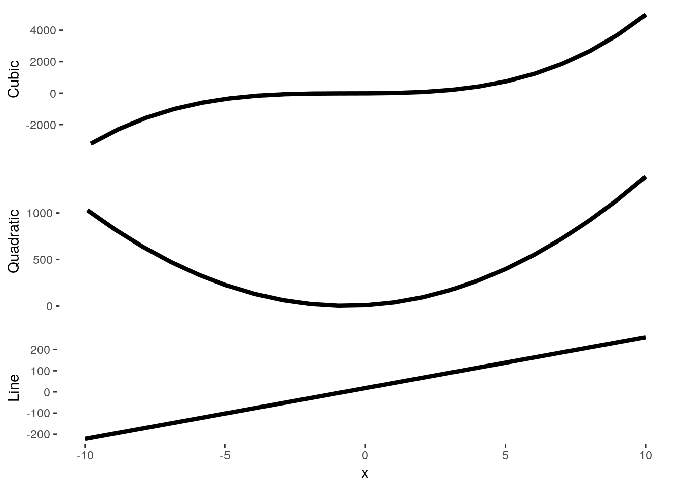

And voila, there you have a plot with a watermark to show off, there are lots of ways to customize these points, for my contract I included axis lines like so

grid.newpage()
grid.draw(quartLine)

print(linePlot + theme(axis.line = element_line(colour = "black")), vp = vp1)
print(quadPlot + theme(axis.line = element_line(colour = "black")), vp = vp2)
print(cubicPlot + theme(axis.line = element_line(colour = "black")), vp = vp3)

For highly technical work it is important to note that the panels will not necessarily be in alignment. For example, because the longest axis label on the cubic plot is a digit longer than the other plots it’s drawing panel (where the plotting happens) is one digit narrower. This can probably be circumvent (though I’ve never tried) by manually specifying the size of the label box in your themes.

Outro

So there is how you can get around some of the limitations of ggplot2 to make really nifty figures for your own work and analyses. If you’re really intrigued, maybe investigate grid more deeply and shed the overhead of ggplot2, or you can delve deeper in how to combine the two to make a tricked-out personalized ggplot2 workflow to make some astonishing figures.

I hope you enjoyed this little journey through the innards of ggplot2.

-Chris