R, LaTeX/LyX, and your scientific workflow

On Workflow models

If you’re anything like me, as time goes on, you forget where a file was, or why you did some critical step in an analysis, or a data cleaning step all of which can be very frustrating and time consuming as you retrace your steps. By integrating our writing and analysis, i.e. workflows, we can make it harder for things to go wrong. So what are the steps involved in a typical science workflow. Here is a generic workflow model (after the reading, hypothesis formation, study design, and field/lab work of course).

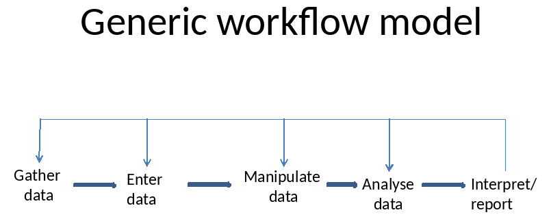
So, how can we tackle this universal problem? I’ll present to you the evolution of my workflow model as special cases of the Generic Model. Here is my original workflow model - it may look rather familiar. (Note that ‘Manipulate data’ is a category for that phase when you are cleaning the data, manipulating it, doing exploratory analysis, and making a bunch of decisions before the formal analysis).

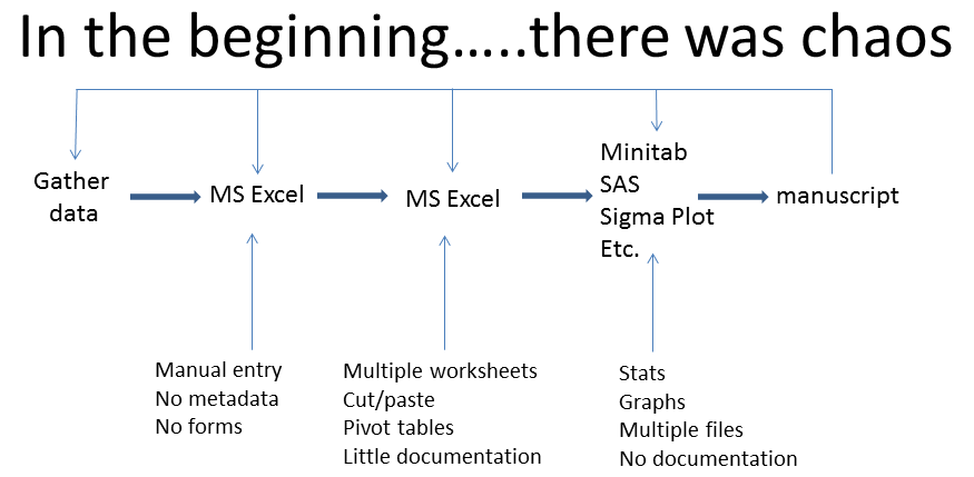
So clearly, this was a bloody mess and is frankly, a bit embarrassing although not all of it was my fault. As biologists, we never really got any training in this area because until fairly recently, large biological data sets weren’t terribly common. Therefore, our mentors usually didn’t know a lot about this stuff, so most of us learned by trial and error. But to briefly elaborate, I had nice data sheets but no systematic way to enter the data into Excel. I’d never head of metadata (data that describes data, e.g. sources, definitions of variables and acronyms). I was pretty good with Excel and formatted my data using a combination of cut/paste, multiple worksheets, and pivot tables. I did my analyses in several packages depending on what was easiest (Minitab, SAS, DataDesk - a wonderful little program). Graphing was done in SigmaPlot (bad, evil, SigmaPlot; the designers are clearly not statisticians familiar with the model based approach). Then, I would write it all up in Word (Perfect!). In addition to the problems I’ve outlined above, having all these tools made it really difficult to become really proficient with any of them. It also made formatting painful but the real trouble began when I had to go back and re-analyze/re-write. The limitations of this approach became obvious. What did that acronym mean? Why did I make that change from the raw data? Why did I use this analysis and not that one? Where are the @#$%&# files and which one of the several versions should I use? Why in ‘choose your deity’ name does SigmaPlot have your format the data in such an asinine way? Etc. Etc. Etc. This approach was, and probably still is, fairly common.

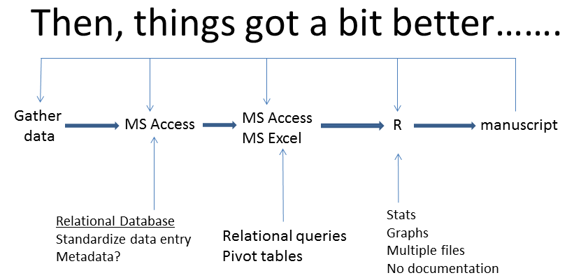
During my PhD, I got a bit smarter and was lucky enough to have Dave Fifield show me how to use relational databases (MS Access) which are vastly superior to spreadsheets for inputting and managing data. Data was well organized, the entry was standardized and the queries in Access are something of a record for how data was manipulated. I won’t talk about this step further but if there is any complexity to your data, or you are setting up a long term research program, do yourself a favour and get it in a database, see this data management paper. But I still didn’t know about metadata and the middle to right side remained a pretty sloppy system. For example, I still had to transfer data from Access to Excel so that I could tweak data for analyses. Even after I moved to R, I really didn’t know much about the data manipulation side of things and all the problems of returning to an analysis and manuscript listed above still apply.

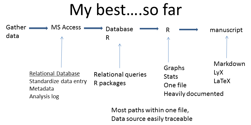
I’m pretty pleased with my current approach In addition to the previous model, I now make sure I have really comprehensive metadata and I save my SQL code (from Access) for each query. I also keep an analysis log writing down all the decisions that I’ve made - there’s nothing worse than thinking hard, for a long time to solve a problem, implementing the solution, only to forget the subtleties 6 months later. Once out of Access, I do all my data manipulation in R (see the dplyr blog; of course I document all the reasons for data manipulation in the code) before preceding to the analyses and graphical output (link to blog on ggplot2).
So suppose you have a good data management system, you’re a whiz with R and reasonably organized. You still need to get your statistical and graphical outputs into a document and format it properly - but Word really sucks for this. The rest of this blog is meant to introduce you to the alphabets soup of tools that can make the right side of the workflow model much, much, easier. The cornerstones of this approach are R (obviously) and LaTeX, the world’s best document preparation system which are linked together by knitr.

Weaving and Knitting

Sweave comes from ‘S’, the precursor to R and you ‘weave’ your analysis into LaTeX just like you ‘knit’ with R (knitr has basically replaced sweave). The idea of ‘weaving’ or ‘knitting’ my R code into a document seemed very practical. The idea came from Donald Knuth’s influential text Literate Programming. His premise was that code needed to be written for humans to understand first, and computers to compile second. By weaving together code and documents you can create a works of code that can be understood much more easily. The idea has broadly fallen out of favour with the main-stream programming communities, although it took root in science. If you can have your analyses bound to your reports, you can save effort lot of time and frustration that I previously described but there are other benefits too!.

Major Difference Between Word and LaTeX

The difference between a word processor and a document preparation system like LaTex is that word processors are what-you-see-is-what-you-get (WYSIWYG) while LaTeX is what-you-see-is-what-you-mean (WYSIWYM). Basically, in a word processor, you have to make it look right on the screen. Some folks are good at this. But if you lack artistic sensibilities (like me), or you just want consistently formatted output that you don’t have to worry too much about it (like me), you need a document preparation system.
In a document preparation system, you write and the computer produces well formatted documents. You usually have to tweak things of course. But the great thing, is that you don’t have to worry about the most of the formatting, i.e. you separate the task of writing from the task of presentation (most of what I’ve read on efficient writing suggests you should separate the tasks of writing, editing, and presentation - for more info see and for something slightly more opinionated. To date, I’ve written lengthy reports with multiple tables and figures. It was a bit of work but formatting hasn’t been anywhere near a problem like in MS Word. To give an example, a few years back when I was learning about this stuff, I was tasked with writing a government report that grew to 180 pages. Formatting was an absolute nightmare. For reasons known only to itself, Word kept italicizing paragraphs, changing headers, etc. Thankfully, I never had to format the bloody thing because unlike a thesis or manuscript, I couldn’t put my tables/figures at the end of a chapter. It would have taken forever! Never again will I use MS Word of my own free will for a complex document! I now do almost all my writing in LaTeX (actually, I use LyX, a GUI for LaTeX - see below). My rule of thumb is that if it’s more than 5-10 pages and has any number of tables or figures, I use LyX!
Formatting is one advantage, but more important for me is the ability to knit my R code with my text and keep track of everything (data manipulation decisions, figures, analyses, etc.). Another advantage to this approach is that you can update reports or papers on the fly (see R and LyX). Suppose you are in the second year of your thesis (this website is a 5 part blog on writing a thesis in LaTeX). Or you are required to submit annual reports for a grant. You have drafted a report or prepared a draft document for publication. Then you have your next field season. With this approach, all you have to do (after entering the data in the proper format of course) is open the document, and re-run the analyses. Of course if this changes your results, you have some work to do but you’d have to do that anyway.

However, there are barriers to learning this approach. LaTeX is code driven and initially, I was in no mood to learn to program for document writing. Fortunately, there is a GUI for LaTeX called LyX. LyX has the look and feel of a word processor but with all the power of LaTeX.

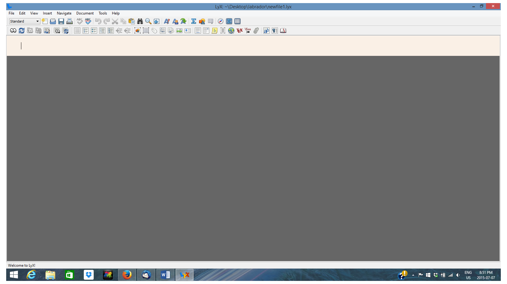
And what is really cool is that LyX can also be integrated (with a little effort) with R and you can produce documents just like Chris has shown in Markdown. More on that below. But if you are not interested in LyX, LaTeX documents can be produced in RStudio (you need to install knitr and then simply File -> New -> R Sweave) or one of the various LaTeX editors like MikTeX (but you are on your own if you choose this path).

Getting Started with R and LyX:

First off, to get started preparing your first LaTeX document, you’ll need to download LyX. This will magically take care of downloading all the LaTeX related software for you. You also need to make sure you’ve installed knitr in R. Once that’s done we need to get LyX talking to R. This website gives good instructions - incidentally, Yihui Xie wrote his entire book ‘Dynamic Documents with R and knitr’ using Lyx and knitr. So a thesis should be a piece of cake!.

Basically, you use chunks just like in Markdown. Write your text just like a word processor. When you want to do an analysis, hit Ctrl-L and an Evil Red Text (ERT) box appears (see below). You then create the R chunk and LyX will embed this analysis in your document. Note that Markdown uses ``` for chunks while LaTeX starts a chunk with <<>>= and ends with @. The following text and code in LyX produces the following output:

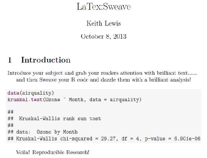
And as mentioned above, if you prefer, you can skip LyX altogether (not sure I recommend this) and do LaTeX right in RStudio just like Chris has done with Markdown. The below will give identical output as the LyX example above. Note that everything following the backslash and in blue font is LaTeX code.

Also, through knitr you have complete control over what does and doesn’t appear in the output.

First the headlines, now the details

OK - that was a very simple introduction but there are some things you need to know before you can really get going. When you open LyX, the first thing you should do is goto Document -> Settings. You should see something like this.

The options in Document Settings are too numerous to blog about but basically, this gives box gives you tremendous flexibility and control over what type of document you create. If you click on Document class, you’ll notice that there are a huge number of document classes to choose from. I usually stick with Article (but see Beamer below). Modules are the way to link to knitr and R (see above).

There is also the format bar the upper left corner (click on ‘Standard’ or Ctl-P). This is required for creating headers and the table of contents. It’s much, much better than Word which again, seems to have a logic known only to its creators. When you are writing your paragraphs, use the ‘Standard’ option - everything else (Section, sub section, paragraph, subparagraph are for the headings).

If you want to see some output, the shortcut is to click on the ‘eyes’ in the upper left corner. Or, you can go to File->export. There’s a lot of options. I usually just use pdflatex.

How do you get your references into LyX?

This was a major barrier for me. There is a built in way to type your references into LyX. Click on the format bar (upper left corner) and select Bibliography. Then you just type your references in old school fashion. But this approach doesn’t format the references as you would in a standard biology journal - at least I never could get it to work. Anyway, for a while, I despaired. Fortunately, Chris figured out BibTeX, the bibliography system for LaTeX and LyX. It’s actually really easy, and citation in LyX is simple. Here’s one method. First, create a simple text file ‘title.bib’. Then, simply Insert -> List/TOC -> BibTeX bibliography in the appropriate part of you text. Click on the Add button and browse your way to your ‘title.bib’ file. Then choose a Style - this controls the format (this will take some experimentation - I often use elsearticle-harv). Then, goto Document -> Settings and click on Bibliography. Under citation style, click ‘Natbib’ and in the ‘Natbib style’ box, click on ‘author-year’ (I’m assuming that most folks want author and year to appear in the text - if you are using the numeric citation, ignore this).

Now you’ll want to add references to the ‘title.bib’ file. Google Scholar can save references at BibTex - goto ‘Settings’ and change Bibliography Manger to BibTeX. Then, find a reference for your paper. There is the option to ‘Import to BibTeX’ under each reference. Click on this and a webpage will appear with something like this:

@article{
  lewis2006statistical,
  title={Statistical power, sample sizes, and the software to calculate them easily},
  author={Lewis, Keith P},
  journal={BioScience},
  volume={56},
  number={7},
  pages={607--612},
  year={2006},
  publisher={Oxford University Press}
}

This is the BibTeX code. Simply copy/paste this to ‘title.bib’. To insert a reference in LyX, simply Insert -> Citation and choose the appropriate reference. You can control the look of the citation by clicking on ‘Citation Style’ under ‘Formatting’. For a how to do BibTeX in LaTeX, see Sharelatex.com.

But of course, you have all your references in a reference manager so here is a more elegant option. Use Zotero with the plugin LyZ which manages BibTeX databases and inserts citation to LyX documents. LyZ allows you to ‘Cite-as-you-write’ in LyX. Here is a link to an excellent pdf by Derek Wolfson that describes how to link these together. It’s fairly straight forward to set up and I’ve used it - highly recommend it!

Conclusion:

In summary, there’s a ‘traditional’ way of handling your workflows. These were the only effective options for the early personal computer age. However, with the rise of R and RStudio, much of this has changed. I hope that this blog has demonstrated that there are readily available tools that can help you work more productively, collaboratively, and reproducibly as a scientist. I hope that this blog will save you some time and effort in learning to use them